Gnuplot - Multiplot

Gnuplot has the option to combine multiple graphs in a layout.  The following picture has the terminology.

• The whole map will be referenced as (0,0) starting with bottom-left, stretching upto (1,1) till top-right.
• If we need to embed a graph inside this layout.  We have to specify the origin of the graph, i.e. where the top left of graph to be placed.  Also, we specify the size, i.e. how much area it is going to occupy.  All this has to be with reference to (0,0) and (1,1) size of multiplot.
• From the picture you can see the margins: left margin(lmargin), right margin(rmargin), top margin(tmargin), bottom margin(bmargin).  These has to be mentioned starting from bottom left position of the layout.

Offset

How much ever we try to plot a layout, there will always be adjustment that has to be done for Labels, tics, titles.  In this case, we use the offset that specifies the alignment of that entity with reference from its default position.  

It definitely takes a trial and error approach to make a desired multiplot.  

Syntax

set multiplot { layout <rows>,<cols>
                {rowsfirst|columnsfirst} {downwards|upwards}
                {title <page title>}
                {scale <xscale>{,<yscale>}}
                {offset <xoff>{,<yoff>}}
              }
unset multiplot

Example

Following are the 4 data files

file1.dat

Time, read1,read2,read3
20,    4.9, 17.1, 78.1 
25,    4.0, 22.0, 74.0 
30,    2.0, 17.0, 81.0 
35,   11.5, 21.7, 66.8 
40,    4.7, 18.0, 77.4 
45,    3.8,  8.9, 87.3 
50,    0.6, 17.3, 82.1 
55,    2.0,  3.4, 94.6 
60,    1.0,  1.3, 97.6 

file2.dat

Time, read1,read2,read3
20,   5.3, 20.6, 74.2
25,   9.2, 27.2, 63.6
30,   9.5, 20.3, 70.2
35,   9.9, 22.1, 68.0
40,   5.3, 19.0, 75.7
45,   3.4,  9.6, 86.9
50,   2.3, 15.3, 82.4
55,   2.7, 10.6, 86.7
60,   1.7,  1.0, 97.3

file3.dat

Time, read1,read2,read3
20,    6.8, 20.6, 72.6
25,    6.2, 29.5, 64.3
30,    5.3, 23.6, 71.1
35,    4.5, 15.6, 79.9
40,    5.5, 17.4, 77.1
45,    3.7, 10.5, 85.8
50,    9.1, 16.6, 74.3
55,    2.8,  3.8, 93.4
60,    1.0,  1.6, 97.4

file4.dat

Time, read1,read2,read3
20,    9.1, 24.2, 66.7
25,    5.1, 26.2, 68.7
30,    9.2, 25.9, 64.9
35,    4.4, 18.4, 77.2
40,    7.6, 17.3, 75.2
45,    4.8,  8.2, 87.0
50,    2.0,  2.1, 95.9
55,    2.6, 10.3, 87.1
60,    2.8,  0.6, 96.6

Script is

1 2 3 4 5 6 7 8 9 10 11 12 13 14 15 16 17 18 19 20 21 22 23 24 25 26 27 28 29 30 31 32 33 34 35 36 37 38 39 40 41 42 43 44 45 46 47 48 49 50 51 52 53 54 55 56 57 58 59 60 61

set terminal pngcairo set output "readings.png" set style data histogram set style histogram rowstacked set yrange [0:100] set xtics 5 set style fill solid set key outside set boxwidth 0.5 relative set datafile separator "," set multiplot layout 4,1 title "MultiArea\nReadings" font ",8" offset 21,0 set ytics border font ",6" offset 0.7,0 set key title 'Readings' font ",6" set key font ",5" set key bottom right set size 1,0.25 set origin 0,0.25 set lmargin at screen 0.1 set tmargin at screen 0.23 set bmargin at screen 0.05 set rmargin at screen 0.85 set title "Area4" font ",6" offset 0,-0.7 set xtics border font ",6" offset 0,0.7 plot for [COL=2:4] 'file4.dat' using COL:xtic(1) ti col unset xtics set size 1,0.25 set origin 0,0.50 set lmargin at screen 0.1 set tmargin at screen 0.48 set bmargin at screen 0.27 set rmargin at screen 0.85 set title "Area3" font ",6" offset 0,-0.7 plot for [COL=2:4] 'file3.dat' using COL:xtic(1) ti col unset key set size 1,0.25 set origin 0,0.75 set lmargin at screen 0.1 set tmargin at screen 0.73 set bmargin at screen 0.52 set rmargin at screen 0.85 set title "Area2" font ",6" offset 0,-0.7 plot for [COL=2:4] 'file2.dat' using COL:xtic(1) ti col set size 1,0.25 set origin 0,0.95 set lmargin at screen 0.1 set tmargin at screen 0.97 set bmargin at screen 0.77 set rmargin at screen 0.85 set title "Area1" font ",6" offset 0,-0.7 plot for [COL=2:4] 'file1.dat' using COL:xtic(1) ti col unset multiplot exit

Going through the steps:

• Line 1-2: The output has to be an image png file
• Lines 4-10: Histogram settings common for all the 4 plots.
• Line 14: Title of the graph.  Offset is used to print it in the top right position.
• Line 17-19: Individual plots key information display settings
• Line 21: The size of the Area4 plot 
• Line 22: The starting position of the Area4 plot
• Line 23-26: Margins of the plot
• Line 27: Title of the plot
• Line 28: Font settings and position of Xtic labels
• Line 29: Setting the plot
• Line 30: Unsetting xtics so that xtic labels do not appear in all the above plots
• Line 32-58: Drawing the other Area plots in the multiplot
• Line 60: End of multiplot
• Line 61: Only after exit is called, the output image file will be ready for viewing

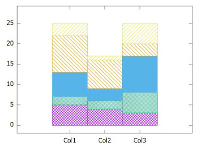
Resultant graph is

Gnuplot - Nonuniform Matrix Data

Nonuniform matrix in Gnuplot refers to a type of data in matrix format.  In this the 

• first row contains the x-coordinate position
• first column contains the y-coordinate position

Lets pick an example matrix and the command.  Lets plot with labels for easier understanding.

num.dat:

  ,1, 2, 4, 5, 7
6, 5, 4, 3, 1, 0
8, 2, 2, 0, 0, 1
3, 0, 0, 0, 1, 0
9, 0, 0, 0, 2, 3
1, 0, 1, 2, 4, 3

Command:

plot 'num.dat' matrix nonuniform using 1:2:(sprintf("%g",$3)) with labels

You can see the command 'matrix nonuniform'.  If we use nonuniform, we explicitly mention it.  If not, it will consider that as uniform.

Now, for making the graph colorful.  Same matrix with palette style 

gnuplot> plot 'num.dat' matrix nonuniform using 1:2:3 \
>with points pointtype 5 pointsize 8 linecolor palette

The different point parameters, make a similar heatmap kind of graph using point type 5(square) and palette.

Gnuplot - Matrix Uniform Data

It is a common Matrix with either rowheader/columnheader and data. Format and example of the matrix with row and column header is 

There may also exists few matrix that doesn't have the headers.  Now, Lets plot it.  Matrix and command

num.dat:

,Apple,Bacon,Cream,Donut,Eclair
Row1, 	5, 4, 3, 1, 0
Row2, 	2, 2, 0, 0, 1
Row3, 	0, 0, 0, 1, 0
Row4, 	0, 0, 0, 2, 3
Row5, 	0, 1, 2, 4, 3

Script:

set datafile separator ","
set palette defined (0 "white", 5 "green")
plot 'num.dat' matrix rowheaders columnheaders  with image

Palette when defined with 0 as white and 5 as green.  It is the basic heatmap.  Any values that are in between will have proportionate white and green colors in them.  Resultant graph will be:

Lets draw a colorful graph.  Here is the data and the script.

num.dat:

,Apple,Bacon,Cream,Donut,Eclair
Row1, 	5, 4, 3, 7, 5
Row2, 	3, 8, 6, 8, 6
Row3, 	6, 7, 5, 7, 5
Row4, 	3, 5, 3, 8, 3
Row5, 	6, 7, 5, 4, 3

Script:

set datafile separator ","
set palette defined (3 "blue",5 "red",8 "green")
plot 'num.dat' matrix rowheaders columnheaders  with image

You see the colorful graph resulted.

NOTE: My palette is defined from 3 to 8.  If your data got any value not within 3 and 8.  The palette adjusts itself and becomes messy like the one below.  Intentionally I inserted 0 in the table and see the palette stretched itself from 0 to 8.

Using 'using'

The following is the demonstration of how we can use 'using' command.  For this purpose we use the uniform matrix without any row or column headers.

num.dat:

5, 4, 3
2, 8, 0

Script:

set datafile separator ","
plot 'num.dat' matrix using 1:2:(sprintf("%g",$3)) with labels

The resultant graph contains the x,y matrix positions as xtics and ytics.The values are printed using sprintf command.

Now, we plot 4 copies of same matrices at 4 different positions.  Labelled with green is the matrix at default position.  Red Labelled will be moved 4 position away from x-axis.  Blue Labelled will be moved 3 positions above from y-axis.  Violet labelled will be moved away both on x-axis and y-axis.  The metric is mentioned in the using command.

plot 'num.dat' matrix using 1:2:(sprintf("%g",$3)) with labels textcolor rgb "green",\
'num.dat' matrix using ($1+4):2:(sprintf("%g",$3)) w labels tc rgb "red",\
'num.dat' matrix using 1:($2+3):(sprintf("%g",$3)) w labels tc rgb "blue",\
'num.dat' matrix using ($1+4):($2+3):(sprintf("%g",$3)) w labels tc rgb "violet"

Result is:

GnuPlot - NewHistogram

NewHistogram, is the command using which we can group histograms into sets.  To demonstrate this, we use the following data files:

num.dat:

    ,Col1,Col2,Col3
Row1,	5,   4,   3
Row2,	2,   2,   5
Row3,	6,   3,   9
Row4,	9,   7,   3
Row5,	3,   1,   5

num2.dat:

    ,2Col1,2Col2,2Col3
2Row1,   7,    3,    5
2Row2,   3,    6,    2
2Row3,   8,    1,    8

Example script to demonstrate

set datafile separator ","
set style data histogram
set style histogram pattern 8
plot newhistogram 'SET 1', for [COL=2:4] 'num.dat' using COL:xtic(1) title column,\
 newhistogram 'SET 2', for [COL=2:4] 'num2.dat' using COL:xtic(1) title column

The command will be like joining two plots together.  We can use line graph or histogram or any other with histogram. Usual syntax will be 'newhistogram <label>'.

In our script we had 2 separate plots.  One for num.dat and other for num2.dat.  We use the prefix 'newhistogram <label>' for both and join it in a single plot.  The resultant graph will be:

GnuPlot - Histogram

Today, we do some plots for histogram. 

We use the following data 'num.dat'

    ,Col1,Col2,Col3
Row1,	5,   4,   3
Row2,	2,   2,   5
Row3,	6,   3,   9
Row4,	9,   7,   3
Row5,	3,   1,   5

Boxes

If a single column plot is needed, 'boxes' will be very helpful. The following commands.

set datafile separator ","
plot 'num.dat' using 2:xtic(1) with boxes fill pattern 5 title column

'using 2' means we plot only column 2.  'xtic(1)' means xtic labels will be from column 1.  The resultant graph will be

Histogram Clustered

Clustered Histogram means putting all the columns side by side.  We plot all the columns in the histogram graph.  The following code:

set datafile separator ","
set style data histogram

set style histogram clustered
set style  fill pattern 4
plot for [COL=2:4] 'num.dat' using COL:xtic(1) title column

• data separator will be comma 
• Setting the style to be histogram and the type clustered.
• Plotting the columns 2 to 4.  Setting the column 1 entries as xtic labels.

Resultant graph will be

Histogram Rowstacked

In Rowstacked the rows are stacked one on top of another.  Like adding the elements of rows. The following code is an example

set datafile separator ","
set style data histogram

set style histogram rowstacked
set style fill pattern 4
plot for [COL=2:4] 'num.dat' using COL:xtic(1) title column

The resultant graph will be

Histogram Columnstacked

In Columnstacked, we stack the columns into towers.  The elements of the column are placed on top of another.

set datafile separator ","
set style data histogram
set style histogram columnstacked
set style  fill pattern 5
plot for [COL=2:4] 'num.dat' using COL title column

• Plot command is different.  We do not use xtics.  Only 'title column' would do the trick.

The resultant graph is 

GnuPlot - Line

Lets put down some of the information related to Line Graph.  The commands and the corresponding graph are displayed in the image.

Line Graph

We can have user defined pattern with characters '_' '.' '-' (underscore, dot, hyphen).  The resultant plot will have big dash for underscore, medium dash for hyphen and small dash for dot.

plot 1 dashtype 1 lw 3, 2 dashtype "_ . - " lw 3

GnuPlot - Points Linepoints Circles

Points

Point Size

Example will be: plot sin(x) with points, sin(x+1) with points pointsize 2, sin(x+2) with points pointsize 4

Point Size

Point Type

Example will be: plot x+1 with points pointtype 1, x+2 w p pt 2, x+3 w p pt 3, x+4 w p pt 4, x+5 w p pt 5

Point Type

If I want to define my own point type, we can use the commands as below:

Lines Point

Point Type

Example command will be: plot sin(x) with linespoint pointtype 6, sin(x+7) w lp pt 7, sin(x+8) w lp pt 8

If I want to have my own symbols, the example will be: 

plot sin(x) with linespoint pt "ß",sin(x+1) with linespoint pt "Y",sin(x+2) with linespoint pt "#"

Circles

For example, we take the following table

x	y	size
1	1	0.6
2	2	0.9
3	3	0.7
4	4	2
5	5	0.9

We overlap the plot with linespoint to understand the relative sizes of circles.  To make this work, the table should always have the third column mentioning the diameter of circles.  The command

gnuplot> set style fill transparent solid 0.2 noborder
gnuplot> plot 'num.dat' using 1:2:3 with circles, 'num.dat' using 1:2:xtic(1) with linespoint

Results in this graph.

Lets take another example, with the following command and the corresponding table.

gnuplot> set style fill transparent solid 0.2 noborder
gnuplot> plot 'num.dat' using 1:2:3 with circles, 'num.dat' using 1:2:xtic(1) with linespoint

PieChart

GnuPlot doesn't support PieChart.

Gnuplot - Tics

Some information regarding Tics is listed in this blog.  We use the following table 'num2.dat'

 

Row    Col1 
Row1    2
Row2    4
Row3    -2
Row4    3

By default, xtics and ytics will denote the position. We can make one of the column display the corresponding values on the x-axis.

Xtics

We can pass different values to the positions from the script.  The syntax is 

set xtics (“<label>” <pos>, …….)

Example for either xtics/ytics are:

set ytics ("Zero" 0, "Four" 4)
set xtics ("NewOne" 1, "NewFour" 4)
plot 'num2.dat' using 2

The graph would look like:

Tics - Script Defined

In any case, the space is not sufficient to display the xtic label, we can rotate the text by mentioning the degree, either clockwise(use minus symbol before degree) or anticlockwise.  We use the command 'rotate by'.

Tics 'Rotate by'

'offset 0,-1.5' means how much we deviate by x-axis and y-axis from its default position.  If we dont use it, the display would be on the line.  Just a minor adjustment.

Gnuplot - Basics

The following pictures could serve as references.

Function Plot

Data File Plots

There are some of the other parameters related to a graph

set grid
set key outside
set xrange [0:10]
set yrange [0:100]
set xtics 1
set ytics 10
set xlabel "number"
set ylabel "square"
set title "Square of the Numbers"
plot x*x

The graph for this script is the following:

Using 'using'

Generally 'using' is to plot columns of a data plot.  The following are 3 ways of representing the same result.

plot 'sta1.dat' using 2:xtic(1) , 'sta1.dat' using 3, 'sta1.dat' using 4 title column, 'sta2.dat' using 3

plot 'sta1.dat' using 2:xtic(1) , '' u 3, '' u 4 ti col, 'sta2.dat' using 3

plot for [COL=2:4] 'sta1.dat' u COL:xtic(1) ti col, 'sta2.dat' u 3

Secondary Axis

We can have secondary axis on the right margin or top margin. The parameters related to those will be starting with x2 or y2 accordingly.  For example x2labels, y2tics, etc.

Here is the example of having two plots with (primary-x-axis, primary-y-axis) and (secondary-x-axis,primary-y-axis) in the same graph.

set xrange [0:10]
set yrange [0:10]
set y2range [-2:2]

set xlabel 'X axis'
set ylabel 'Y axis'
set y2label 'Y2 axis'
set y2tics 1

plot 2*x axes x1y1, sin(x) axes x1y2

The resultant graph is 'sec-axis-1'

Sec-axis-1

The following is another script the uses (primary-x-axis,primary-y-axis) and (secondary-x-axis,secondary-y-axis).

set x2range [-20:20]
set xrange [-10:10]
set y2range [-3:3]
set yrange [-1:1]

set y2tics 1
set x2tics 4

set xlabel "X1 Axis"
set ylabel "Y1 Axis"
set x2label "X2 Axis"
set y2label "Y2 Axis"

plot sin(x) axes x1y1 title "X1-Y1 Axis", cos(x) axes x2y2 title "X2-Y2 Axis"

The resultant graph will be

Sec-axis-2